Suppose f(x) and g(t) are two functions of real numbers. Their convolution is defined by
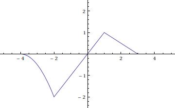
Let's look at an example. Here we have chosen a function f(x) that vanishes except for x values in this window.
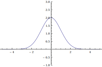
We will convolve f with a gaussian function g(t)=2e^{-t^2/2}
First, let's look at a Riemann sum approximation of the convolution of f and g. We will use sample points at t=-2,-1,0,1,2 .
Here is an animation of the multiples of translations of f(x) that we will add together to form our Riemann sum approximation of the convolution f \ast g (x) .
Adding the functions from each frame in the animation above gives us the following Riemann sum approximation for the convolution.
Now compare this to a true plot of the convolution f \ast g (x) .